Puncta Segmentation

This notebook demonstrates how to segment puncta from an image using the “Analyze Particles” ImageJ plugin, perform measurements and return those values as a pandas DataFrame.

First let’s initialize ImageJ in headless mode with the legacy layer enabled. See How to initialize PyImageJ for more information on PyImageJ’s initialization modes.

import imagej
import scyjava as sj

# initialize imagej
ij = imagej.init(mode='headless', add_legacy=True)
print(f"ImageJ version: {ij.getVersion()}")

ImageJ version: 2.14.0/1.54f

Now that ImageJ has been successfully initialized, let’s next import the Java classes (i.e. ImageJ resources) we need for the rest of the workflow.

# get additional resources
HyperSphereShape = sj.jimport('net.imglib2.algorithm.neighborhood.HyperSphereShape')
Overlay = sj.jimport('ij.gui.Overlay')
Table = sj.jimport('org.scijava.table.Table')
ParticleAnalyzer = sj.jimport('ij.plugin.filter.ParticleAnalyzer')

Next we load the data with ij.io().open() and then convert the 16-bit image to 32-bit with ImageJ ops (i.e. ij.op().convert().int32()). Alternatively you can load the data using other software packages such as scikit-image’s skimage.io.imread() which returns a NumPy array. To convert the NumPy array into an ImageJ Java image (e.g. a Dataset: net.imagej.Dataset) call ij.py.to_dataset().

The sample images used in this notebook are available on the PyImageJ GitHub repository here.

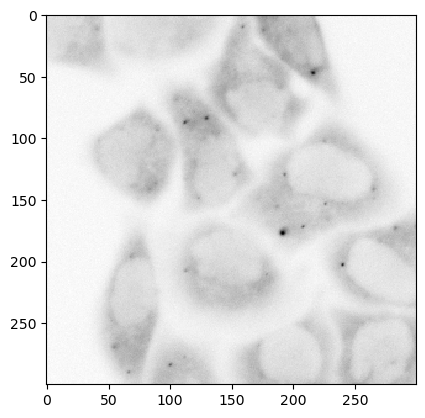
# load test data
ds_src = ij.io().open('sample-data/test_still.tif')
ds_src = ij.op().convert().int32(ds_src) # convert image to 32-bit
ij.py.show(ds_src, cmap='binary')

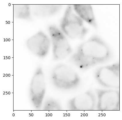
There are many ways to background subtract/supress noise in an image. In this example we take a duplicate of the input image, here ds_mean, apply a mean filter with a radius of 5 and then multiply it back to the original image. The trick to this operation improving the signal-to-noise ratio lies in the application of the mean filter. In the background area outside of the cell high value pixels are generally intermixed with low value ones. In contrast the high value pixels in the object of interest are surrounded by high value ones. When the mean filter is applied, the high value pixels in the background are averaged with low values and high values pixels in the object are averaged with other high value pixels. When this mean filtered image is multiplied with the original image, the background noise is multiplied by a “smaller” number than the objects/signal of interest. Note that these are destructive changes and the resulting background supressed image is not sutible for measurements. Instead, these processes are done to generate masks and labels which can then be applied over the original data to obtain measurements that are unmodified.

Here we are using ImageJ ops to apply the mean filter. You can also apply the filter using ij.py.run_plugin(imp, "Mean...", "radius=2"). Note that using the original ImageJ plugins/functions like “Mean…” require the ImagePlus image data type. In this case we can convert the ds_mean into an ImagePlus like so:

imp = ij.py.to_imageplus(ds_mean)

# supress background noise
mean_radius = HyperSphereShape(5)
ds_mean = ij.dataset().create(ds_src.copy())
ij.op().filter().mean(ds_mean, ds_src.copy(), mean_radius)
ds_mul = ds_src * ds_mean
ij.py.show(ds_mul, cmap='binary')

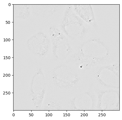
Here we employ a gaussian blur subtraction to futher enhance the puncta for segmentation. For more information on gaussian blurs and how they can be used in image processing please checkout Peter Bankhead’s amazing online book.

# use gaussian subtraction to enhance puncta
img_blur = ij.op().filter().gauss(ds_mul.copy(), 1.2)
img_enhanced = ds_mul - img_blur
ij.py.show(img_enhanced, cmap='binary')

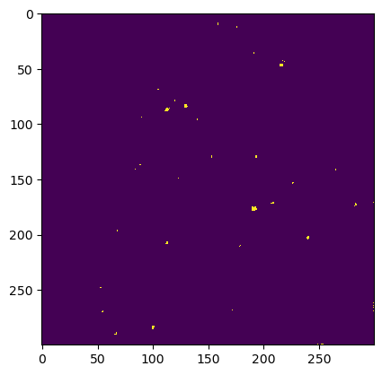
# apply threshold
img_thres = ij.op().threshold().renyiEntropy(img_enhanced)
ij.py.show(img_thres)

Finally we convert the threshold image into an ImagePlus with ij.py.to_imageplus() and run the “Analyze Particles” plugin. The ResultsTable that is returned by the “Analyze Particles” plugin first needs to be converted to a SciJava table (i.e. org.scijava.table.Table) before it can be converted to a pandas DataFrame.

# convert ImgPlus to ImagePlus
imp_thres = ij.py.to_imageplus(img_thres)

# tell ImageJ to use a black background
Prefs = sj.jimport('ij.Prefs')
Prefs.blackBackground = True

# get ResultsTable and set ParticleAnalyzer
rt = ij.ResultsTable.getResultsTable()
ParticleAnalyzer.setResultsTable(rt)

# set measurements
ij.IJ.run("Set Measurements...", "area center shape")

# run the analyze particle plugin
ij.py.run_plugin(plugin="Analyze Particles...", args="clear", imp=imp_thres)

# convert results table -> scijava table -> pandas dataframe
sci_table = ij.convert().convert(rt, Table)
df = ij.py.from_java(sci_table)

Operating in headless mode - the original ImageJ will have limited functionality.
Operating in headless mode - the ResultsTable class will not be fully functional.
Operating in headless mode - the IJ class will not be fully functional.

# print dataframe
df

	Area	XM	YM	Circ.	AR	Round	Solidity
0	2.0	159.500000	10.000000	1.000000	2.000000	0.500000	1.000000
1	2.0	176.500000	13.000000	1.000000	2.000000	0.500000	1.000000
2	1.0	191.500000	36.500000	1.000000	1.000000	1.000000	1.000000
3	1.0	217.500000	43.500000	1.000000	1.000000	1.000000	1.000000
4	1.0	219.500000	44.500000	1.000000	1.000000	1.000000	1.000000
5	9.0	216.500000	47.500000	1.000000	1.000000	1.000000	1.000000
6	1.0	105.500000	69.500000	1.000000	1.000000	1.000000	1.000000
7	1.0	120.500000	79.500000	1.000000	1.000000	1.000000	1.000000
8	7.0	130.214286	84.500000	1.000000	1.068847	0.935588	0.875000
9	8.0	113.375000	87.625000	0.620562	2.250157	0.444413	0.727273
10	1.0	90.500000	94.500000	1.000000	1.000000	1.000000	1.000000
11	1.0	140.500000	96.500000	1.000000	1.000000	1.000000	1.000000
12	2.0	153.500000	130.000000	1.000000	2.000000	0.500000	1.000000
13	4.0	194.000000	130.000000	1.000000	1.000000	1.000000	1.000000
14	2.0	89.000000	137.500000	1.000000	2.000000	0.500000	1.000000
15	1.0	84.500000	141.500000	1.000000	1.000000	1.000000	1.000000
16	2.0	265.500000	142.000000	1.000000	2.000000	0.500000	1.000000
17	1.0	123.500000	149.500000	1.000000	1.000000	1.000000	1.000000
18	3.0	226.833333	153.833333	1.000000	1.463849	0.683130	0.857143
19	5.0	208.700000	172.100000	1.000000	1.552986	0.643921	0.909091
20	1.0	299.500000	171.500000	1.000000	1.000000	1.000000	1.000000
21	4.0	283.500000	173.500000	0.698132	1.581137	0.632456	0.615385
22	15.0	192.100000	177.033333	0.803786	1.233468	0.810723	0.833333
23	2.0	68.500000	197.000000	1.000000	2.000000	0.500000	1.000000
24	6.0	240.666667	203.333333	1.000000	1.290994	0.774597	0.800000
25	3.0	113.166667	208.166667	1.000000	1.463849	0.683130	0.857143
26	2.0	179.000000	211.000000	0.785398	2.645750	0.377965	0.666667
27	1.0	53.500000	248.500000	1.000000	1.000000	1.000000	1.000000
28	1.0	299.500000	262.500000	1.000000	1.000000	1.000000	1.000000
29	1.0	299.500000	264.500000	1.000000	1.000000	1.000000	1.000000
30	1.0	299.500000	266.500000	1.000000	1.000000	1.000000	1.000000
31	1.0	172.500000	268.500000	1.000000	1.000000	1.000000	1.000000
32	3.0	55.166667	270.166667	1.000000	1.463849	0.683130	0.857143
33	1.0	299.500000	269.500000	1.000000	1.000000	1.000000	1.000000
34	5.0	100.900000	284.300000	1.000000	1.552986	0.643921	0.909091
35	3.0	67.166667	290.166667	1.000000	1.463849	0.683130	0.857143
36	1.0	249.500000	299.500000	1.000000	1.000000	1.000000	1.000000
37	3.0	253.500000	299.500000	0.967374	3.000000	0.333333	1.000000