Classic Segmentation
In this notebook, we will segment the cells image using a traditional ImageJ segmentation workflow:
Preprocess the image
Apply an auto threshold
Create and manipulate a mask
Create and transfer a selection from the mask to the original image
Analyze the resulting data
|
💡 See the “Segmentation with ImageJ” living workshop for a primer on segmentation in ImageJ. |
We will do the same analysis twice: once with ImageJ, and then again with ImageJ2.
Segmentation workflow with original ImageJ functions
import imagej
import scyjava as sj

# initialize ImageJ
ij = imagej.init('sc.fiji:fiji', mode='interactive')
print(f"ImageJ version: {ij.getVersion()}")
ImageJ version: 2.9.0/1.53t
WARNING: An illegal reflective access operation has occurred
WARNING: Illegal reflective access by sc.fiji.compat.DefaultFijiService (file:/home/gselzer/.jgo/sc.fiji/fiji/RELEASE/6036d0a247032b7c753533e176fb5178354d75af4ac706eaf88adac9c1ccb068/fiji-2.9.0.jar) to field sun.awt.X11.XToolkit.awtAppClassName
WARNING: Please consider reporting this to the maintainers of sc.fiji.compat.DefaultFijiService
WARNING: Use --illegal-access=warn to enable warnings of further illegal reflective access operations
WARNING: All illegal access operations will be denied in a future release
import skimage
cells = skimage.data.cells3d()
Because this sample image is a NumPy array, but not an xarray, it does not have dimensional axis labels. However, scikit-image has defined conventions for the order of dimensions as follows:
(t, pln, row, col, ch)
Where t is time, pln is plane/Z, row is row/Y, col is column/X, and ch is channel.
Now that we are armed with that knowledge, notice that cells actually has a slightly different dimension order, with planar rather than interleaved channels: (pln, ch, row, col). Let’s construct an xarray from this image that includes the correct dimensional axis labels:
import xarray
xcells = xarray.DataArray(cells, name='xcells', dims=('pln', 'ch', 'row', 'col'))

# print some basic info
print(f"name: {xcells.name}\ndimensions: {xcells.dims}\nshape: {xcells.shape}")
name: xcells
dimensions: ('pln', 'ch', 'row', 'col')
shape: (60, 2, 256, 256)
# convert xcells image to ImagePlus
imp = ij.py.to_imageplus(xcells)
imp.setTitle("cells")
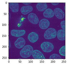
# slice out an image plane.
c, z, t = 2, 36, 1
Duplicator = sj.jimport('ij.plugin.Duplicator')
imp2d = Duplicator().run(imp, c, c, z, z, t, t)
imp2d.setTitle("cells-slice")
ij.py.show(imp2d)
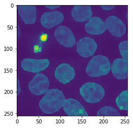
# preprocess with edge-preserving smoothing
ij.IJ.run(imp2d, "Kuwahara Filter", "sampling=10") # Look ma, a Fiji plugin!
ij.py.show(imp2d)
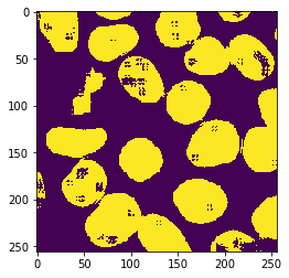
# threshold to binary mask
Prefs = sj.jimport('ij.Prefs')
Prefs.blackBackground = True
ij.IJ.setAutoThreshold(imp2d, "Otsu dark")
ImagePlus = sj.jimport("ij.ImagePlus")
mask = ImagePlus("cells-mask", imp2d.createThresholdMask())
ij.IJ.run(imp2d, "Close", "")
ij.py.show(mask)
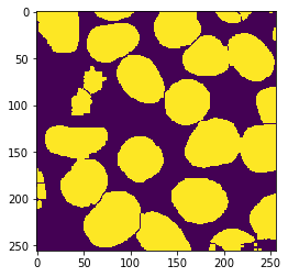
# clean up the binary mask.
ij.IJ.run(mask, "Dilate", "")
ij.IJ.run(mask, "Fill Holes", "")
ij.IJ.run(mask, "Watershed", "")
ij.py.show(mask)
# Save the mask as a selection (a.k.a. ROI).
ij.IJ.run(mask, "Create Selection", "")
roi = mask.getRoi()
ij.IJ.run(mask, "Close", "")

# Split the ROI into cells.
# This works because cells are disconnected due to the watershed.
rois = roi.getRois()
print(len(rois), "cells detected")
32 cells detected
# Calculate statistics.

from collections import defaultdict
from pandas import DataFrame

# Make sure to measure the same slice as segmented!
imp.setPosition(c, z, t)

# Measure each cell, accumulating results into a dictionary.
ij.IJ.run("Set Measurements...", "area mean min centroid median skewness kurtosis redirect=None decimal=3");
results = ij.ResultsTable.getResultsTable()
stats_ij = defaultdict(list)
for cell in rois:
    imp.setRoi(cell)
    ij.IJ.run(imp, "Measure", "")
    for column in results.getHeadings():
        stats_ij[column].append(results.getColumn(column)[0])
# Display the results.
df_ij = DataFrame(stats_ij)
df_ij
| (A, r, e, a) | (M, e, a, n) | (M, i, n) | (M, a, x) | (X) | (Y) | (M, e, d, i, a, n) | (S, k, e, w) | (K, u, r, t) | |
|---|---|---|---|---|---|---|---|---|---|
| 0 | 8.0 | 14267.75 | 12045.0 | 16929.0 | 251.0 | 1.0 | 14748.0 | 0.120347 | -1.164583 |
| 1 | 8.0 | 14267.75 | 12045.0 | 16929.0 | 251.0 | 1.0 | 14748.0 | 0.120347 | -1.164583 |
| 2 | 8.0 | 14267.75 | 12045.0 | 16929.0 | 251.0 | 1.0 | 14748.0 | 0.120347 | -1.164583 |
| 3 | 8.0 | 14267.75 | 12045.0 | 16929.0 | 251.0 | 1.0 | 14748.0 | 0.120347 | -1.164583 |
| 4 | 8.0 | 14267.75 | 12045.0 | 16929.0 | 251.0 | 1.0 | 14748.0 | 0.120347 | -1.164583 |
| 5 | 8.0 | 14267.75 | 12045.0 | 16929.0 | 251.0 | 1.0 | 14748.0 | 0.120347 | -1.164583 |
| 6 | 8.0 | 14267.75 | 12045.0 | 16929.0 | 251.0 | 1.0 | 14748.0 | 0.120347 | -1.164583 |
| 7 | 8.0 | 14267.75 | 12045.0 | 16929.0 | 251.0 | 1.0 | 14748.0 | 0.120347 | -1.164583 |
| 8 | 8.0 | 14267.75 | 12045.0 | 16929.0 | 251.0 | 1.0 | 14748.0 | 0.120347 | -1.164583 |
| 9 | 8.0 | 14267.75 | 12045.0 | 16929.0 | 251.0 | 1.0 | 14748.0 | 0.120347 | -1.164583 |
| 10 | 8.0 | 14267.75 | 12045.0 | 16929.0 | 251.0 | 1.0 | 14748.0 | 0.120347 | -1.164583 |
| 11 | 8.0 | 14267.75 | 12045.0 | 16929.0 | 251.0 | 1.0 | 14748.0 | 0.120347 | -1.164583 |
| 12 | 8.0 | 14267.75 | 12045.0 | 16929.0 | 251.0 | 1.0 | 14748.0 | 0.120347 | -1.164583 |
| 13 | 8.0 | 14267.75 | 12045.0 | 16929.0 | 251.0 | 1.0 | 14748.0 | 0.120347 | -1.164583 |
| 14 | 8.0 | 14267.75 | 12045.0 | 16929.0 | 251.0 | 1.0 | 14748.0 | 0.120347 | -1.164583 |
| 15 | 8.0 | 14267.75 | 12045.0 | 16929.0 | 251.0 | 1.0 | 14748.0 | 0.120347 | -1.164583 |
| 16 | 8.0 | 14267.75 | 12045.0 | 16929.0 | 251.0 | 1.0 | 14748.0 | 0.120347 | -1.164583 |
| 17 | 8.0 | 14267.75 | 12045.0 | 16929.0 | 251.0 | 1.0 | 14748.0 | 0.120347 | -1.164583 |
| 18 | 8.0 | 14267.75 | 12045.0 | 16929.0 | 251.0 | 1.0 | 14748.0 | 0.120347 | -1.164583 |
| 19 | 8.0 | 14267.75 | 12045.0 | 16929.0 | 251.0 | 1.0 | 14748.0 | 0.120347 | -1.164583 |
| 20 | 8.0 | 14267.75 | 12045.0 | 16929.0 | 251.0 | 1.0 | 14748.0 | 0.120347 | -1.164583 |
| 21 | 8.0 | 14267.75 | 12045.0 | 16929.0 | 251.0 | 1.0 | 14748.0 | 0.120347 | -1.164583 |
| 22 | 8.0 | 14267.75 | 12045.0 | 16929.0 | 251.0 | 1.0 | 14748.0 | 0.120347 | -1.164583 |
| 23 | 8.0 | 14267.75 | 12045.0 | 16929.0 | 251.0 | 1.0 | 14748.0 | 0.120347 | -1.164583 |
| 24 | 8.0 | 14267.75 | 12045.0 | 16929.0 | 251.0 | 1.0 | 14748.0 | 0.120347 | -1.164583 |
| 25 | 8.0 | 14267.75 | 12045.0 | 16929.0 | 251.0 | 1.0 | 14748.0 | 0.120347 | -1.164583 |
| 26 | 8.0 | 14267.75 | 12045.0 | 16929.0 | 251.0 | 1.0 | 14748.0 | 0.120347 | -1.164583 |
| 27 | 8.0 | 14267.75 | 12045.0 | 16929.0 | 251.0 | 1.0 | 14748.0 | 0.120347 | -1.164583 |
| 28 | 8.0 | 14267.75 | 12045.0 | 16929.0 | 251.0 | 1.0 | 14748.0 | 0.120347 | -1.164583 |
| 29 | 8.0 | 14267.75 | 12045.0 | 16929.0 | 251.0 | 1.0 | 14748.0 | 0.120347 | -1.164583 |
| 30 | 8.0 | 14267.75 | 12045.0 | 16929.0 | 251.0 | 1.0 | 14748.0 | 0.120347 | -1.164583 |
| 31 | 8.0 | 14267.75 | 12045.0 | 16929.0 | 251.0 | 1.0 | 14748.0 | 0.120347 | -1.164583 |
Notice that we avoided using the RoiManager, so that the workflow still works in headless mode.
Segmentation workflow with ImageJ2
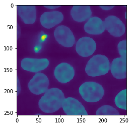
# slice out an image plane.
c, z = 1, 35
cells_slice = xcells[z,c,:,:]
ij.py.show(cells_slice)
jslice = ij.py.to_java(cells_slice)
# preprocess with edge-preserving smoothing.
HyperSphereShape = sj.jimport("net.imglib2.algorithm.neighborhood.HyperSphereShape")
smoothed = ij.op().run("create.img", jslice)
ij.op().run("filter.median", ij.py.jargs(smoothed, cells_slice, HyperSphereShape(5)))
ij.py.show(smoothed)
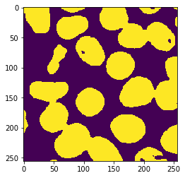
# threshold to binary mask.
mask = ij.op().run("threshold.otsu", smoothed)
ij.py.show(mask)
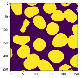
# clean up the binary mask.
mask = ij.op().run("morphology.dilate", mask, HyperSphereShape(1))
mask = ij.op().run("morphology.fillHoles", mask)
ij.py.show(mask)
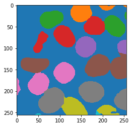
# Watershed: mask to labeling.
use_eight_connectivity = True
draw_watersheds = False
sigma = 10
args = ij.py.jargs(None, mask, use_eight_connectivity, draw_watersheds, sigma, mask)
labeling = ij.op().run("image.watershed", args)
ij.py.show(labeling.getIndexImg(), cmap='tab10')
# calculate statistics.

from collections import defaultdict
from pandas import DataFrame

Regions = sj.jimport("net.imglib2.roi.Regions")
LabelRegions = sj.jimport("net.imglib2.roi.labeling.LabelRegions")

def compute_stats(region, img, stats):
    samples = Regions.sample(region, img)
    stats["area"].append(ij.op().run("stats.size", samples).getRealDouble())
    stats["mean"].append(ij.op().run("stats.mean", samples).getRealDouble())
    min_max = ij.op().run("stats.minMax", samples)
    stats["min"].append(min_max.getA().getRealDouble())
    stats["max"].append(min_max.getB().getRealDouble())
    centroid = ij.op().run("geom.centroid", region)
    stats["centroid"].append(tuple(centroid.getDoublePosition(d) for d in range(centroid.numDimensions())))
    stats["median"].append(ij.op().run("stats.median", samples).getRealDouble())
    stats["skewness"].append(ij.op().run("stats.skewness", samples).getRealDouble())
    stats["kurtosis"].append(ij.op().run("stats.kurtosis", samples).getRealDouble())

regions = LabelRegions(labeling)
stats_ops = defaultdict(list)
for region in regions:
    compute_stats(region, jslice, stats_ops)
df_ops = DataFrame(stats_ops)
df_ops
| area | mean | min | max | centroid | median | skewness | kurtosis | |
|---|---|---|---|---|---|---|---|---|
| 0 | 1860.0 | 14358.090860 | 2845.0 | 30918.0 | (238.75, 143.9758064516129) | 14368.0 | 0.129771 | 3.085133 |
| 1 | 1869.0 | 16544.414660 | 3177.0 | 55766.0 | (132.11824505082933, 237.0904226859283) | 16028.0 | 0.846920 | 5.862000 |
| 2 | 2728.0 | 13762.175953 | 3841.0 | 36656.0 | (81.17192082111437, 222.23717008797655) | 13183.0 | 0.795826 | 4.241153 |
| 3 | 2445.0 | 14010.395092 | 3414.0 | 32483.0 | (188.73824130879345, 141.48711656441716) | 13704.0 | 0.454090 | 3.666324 |
| 4 | 2364.0 | 15095.145516 | 3367.0 | 38648.0 | (173.9784263959391, 201.498730964467) | 14700.0 | 0.560561 | 3.622262 |
| 5 | 1688.0 | 11611.678318 | 4220.0 | 24801.0 | (24.873815165876778, 19.488744075829384) | 11476.0 | 0.413529 | 3.775973 |
| 6 | 1652.0 | 12272.721550 | 4884.0 | 22525.0 | (149.73365617433413, 18.008474576271187) | 12045.0 | 0.339055 | 3.104162 |
| 7 | 1077.0 | 19755.374188 | 3841.0 | 49365.0 | (243.6146703806871, 220.35468895078924) | 18968.0 | 0.403299 | 3.173040 |
| 8 | 1894.0 | 13802.092397 | 3936.0 | 29306.0 | (160.63991552270326, 96.76663146779303) | 13704.0 | 0.090845 | 3.354490 |
| 9 | 1952.0 | 12997.042008 | 3557.0 | 32720.0 | (51.01485655737705, 183.14241803278688) | 12661.0 | 0.522687 | 3.443799 |
| 10 | 1889.0 | 16312.916887 | 4315.0 | 35186.0 | (110.6913710958179, 157.39332980412917) | 16170.0 | 0.295547 | 3.487587 |
| 11 | 1912.0 | 12057.073745 | 5121.0 | 29543.0 | (111.23640167364017, 72.53190376569037) | 11831.5 | 0.592143 | 4.013051 |
| 12 | 1857.0 | 11899.947765 | 4600.0 | 23331.0 | (228.12493268712979, 48.758212170166935) | 11760.0 | 0.405282 | 3.393002 |
| 13 | 1707.0 | 14147.489748 | 4268.0 | 28500.0 | (181.02929115407147, 48.438195664909195) | 14084.0 | 0.093980 | 3.090271 |
| 14 | 1772.0 | 12716.510722 | 4315.0 | 27409.0 | (80.12810383747178, 32.261851015801355) | 12519.0 | 0.696379 | 4.398843 |
| 15 | 595.0 | 14126.727731 | 4837.0 | 36846.0 | (246.10588235294117, 97.0890756302521) | 13657.0 | 1.145941 | 6.003222 |
| 16 | 1922.0 | 15867.754422 | 4410.0 | 41113.0 | (41.289281997918835, 138.36732570239334) | 15838.0 | 0.401893 | 4.441288 |
| 17 | 807.0 | 11452.887237 | 3841.0 | 23236.0 | (210.40644361833952, 244.70755885997522) | 11049.0 | 0.647504 | 3.617672 |
| 18 | 302.0 | 11532.900662 | 5785.0 | 17925.0 | (82.06622516556291, 3.4768211920529803) | 11594.5 | -0.122937 | 2.561317 |
| 19 | 69.0 | 12439.275362 | 3936.0 | 22525.0 | (188.2463768115942, 252.02898550724638) | 12377.0 | 0.160562 | 2.404485 |
| 20 | 1.0 | 9247.000000 | 9247.0 | 9247.0 | (195.0, 253.0) | 9247.0 | NaN | NaN |
| 21 | 938.0 | 21366.135394 | 5027.0 | 58754.0 | (55.124733475479744, 85.94456289978677) | 16858.0 | 0.884682 | 2.610502 |
| 22 | 7.0 | 10391.857143 | 6544.0 | 14843.0 | (230.0, 242.0) | 10622.0 | -0.013143 | 1.421185 |
| 23 | 344.0 | 11232.008721 | 4884.0 | 17783.0 | (209.86627906976744, 4.953488372093023) | 11333.0 | -0.090939 | 2.805479 |
| 24 | 32.0 | 11217.812500 | 6876.0 | 15459.0 | (50.125, 254.15625) | 11618.0 | -0.200546 | 1.948018 |
| 25 | 68.0 | 13067.132353 | 5216.0 | 22620.0 | (253.4264705882353, 24.176470588235293) | 13182.5 | -0.210502 | 2.198048 |
| 26 | 234.0 | 10364.376068 | 5928.0 | 20201.0 | (2.7051282051282053, 189.76495726495727) | 10053.0 | 0.733560 | 4.018682 |
| 27 | 31.0 | 12326.258065 | 5453.0 | 16929.0 | (252.41935483870967, 1.7741935483870968) | 12472.0 | -0.574606 | 2.739545 |