3D Deconvolution

In this notebook, we will perform Richardson-Lucy (RL) deconvolution on a 3D dataset with PyImageJ and imagej-ops. To learn more about deconvolution please visit the RL deconvolution wikipedia page and the imagej.net wiki page on deconvolution.

This example uses a 3D image (shape: (200, 200, 61)) of a HeLa cell nucleus stained with DAPI (4′,6-diamidino-2-phenylindole) and imaged on an epifluorescent microscope at 100x. Although the imagej-ops framework implements the standard RL algorithm, this notebook utilizes the Richardson-Lucy Total Variation (RLTV) algorithm, which uses a regularization factor to limit the noise amplified by the RL algorithm¹.

Richardson-Lucy Total Variation Deconvolution with ImageJ2 and imagej-ops

While it’s not necessary to specify add_legacy=False for this workflow (initializing imagej with ij = imagej.init() works equally as well), legacy is disabled here to demonstrate that this workflow only needs imagej2 and the imagej-ops framework.

Let’s start by first initializing ImageJ2.

import imagej
import matplotlib.pyplot as plt

ij = imagej.init(add_legacy=False)
print(f"ImageJ2 version: {ij.getVersion()}")

ImageJ2 version: 2.14.0

Now, let’s load the sample data and display slice 30.

# open the 3D HeLa dataset
img = ij.io().open('https://media.imagej.net/workshops/data/3d/hela_nucleus.tif')

# display slice 30 of the dataset
ij.py.show(img[:, :, 30])

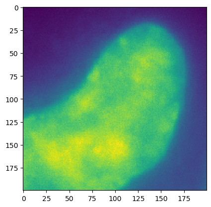
Here we can see a fuzzy slice of the HeLa nucleus. The next few cells will set up the needed components to run RLTV on the 3D datasets. The RLTV implementation in the imagej-ops framework requires four parameters:

• input image (32-bit)

• point spread function (synthetic or real)

• iterations

• regularization factor

The input image is the original image img. The point spread function (PSF) can be either real (i.e. a collected PSF) or synthetic. This notebook will create a synthetic PSF using imagej-ops. iterations is the number of times the data is deconvolved (note: higher iteration values may introduce processing artifacts). The regularization factor reduces the noise amplified by the RL algorithm. Higer values result in greater noise suppression. For now lets set the number of iterations to 15 and the regularization factor to 0.002 (this value is derived from the Dey et. al paper).

# set the iterations and regularization factor for Richardson-Lucy TV
iterations = 15
reg = 0.002

Creating a synthetic PSF with the Gibson-Lanni model.

The next cell will set the parameters needed to generate the synthetic point spread function (PSF) we need to deconvolve the input image. These values are derived from your experimental parameters. For this dataset the needed values are:

Parameter	Value
Numerical Aperture	1.45
Emission Wavelength	457 nm
Refractive index (immersion)	1.5
Refractive index (sample)	1.4
Lateral resolution (XY)	0.065 μm/pixel
Axial resolution (z)	0.1 μm/pixel
Particle position	0 μm

The numerical aperture can be obtained from the objective used to image the sample, here 1.45. The emission wavelength is the emission wavelength imaged, in this case DAPI’s peak emission wavelength is 457 nm. The refractive index (immersion) and refractive index (sample) are experimentally obtained, however some reasonable average values are 1.5 and 1.4 respectively. The lateral resolution is the μm/pixel value for the given image. The axial resolution is the μm/pixel value for the given image, often the “step size” of a Z acquisition. Lastly, particle position is the distance from the coverslip for the position or point of focus (e.g. if you were imaging a fluorescent bead, the particle position value is how far in μm the sample/bead is away from the coverslip).

na = 1.45 # numerical aperture
wv = 457 # emission wavelength
ri_immersion = 1.5 # refractive index (immersion)
ri_sample = 1.4 # refractive index (sample)
lat_res = 0.065 # lateral resolution (i.e. xy)
ax_res = 0.1 # axial resolution (i.e. z)
pz = 0 # distance away from coverslip

The imagej-ops framework can create a synthetic PSF using the Gibson-Lanni algorithm². To create the synthetic PSF we need to use the kernelDiffraction op in the create namespace. Due to an existing known bug, we need to manually obtain the create namespace. See this troubleshooting section for more information. Before we can use the kernelDiffraction op we also need the net.imglib2.FinalDimensions Java class to create a set of imglib2 dimensions and the net.imglib2.type.numeric.real.FloatType Java class.

# import imagej2 and imglib2 Java classes
CreateNamespace = imagej.sj.jimport('net.imagej.ops.create.CreateNamespace')
FinalDimensions = imagej.sj.jimport('net.imglib2.FinalDimensions')
FloatType = imagej.sj.jimport('net.imglib2.type.numeric.real.FloatType')

The kernelDiffraction op accepts its parameters in meters and not μm or nm. The following cell will convert in required parameters into meters.

# convert input parameters into meters
wv = wv * 1E-9
lat_res = lat_res * 1E-6
ax_res = ax_res * 1E-6
pz = pz * 1E-6

Finally, the kernelDiffraction op requires imglib2 dimensions, which is a Java object (net.imglib2.FinalDimensions), for the PSF. These dimensions are the same as the input image’s dimensions and simply requires casting the image’s shape with FinalDimensions.

# convert the input image dimensions to imglib2 FinalDimensions
psf_dims = FinalDimensions(img.shape)

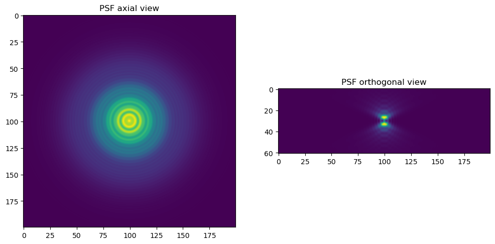
Now with all the parameters set, we can create the PSF and display an axial and orthogonal side view.

# create synthetic PSF
psf = ij.op().namespace(CreateNamespace).kernelDiffraction(psf_dims, na, wv, ri_sample, ri_immersion, lat_res, ax_res, pz, FloatType())

# convert PSF from Java to Python (numpy array)
psf_narr = ij.py.from_java(psf)

# display the axial and orthogonal side view of the PSF side by side
fig, ax = plt.subplots(1, 2, figsize=(12, 9))
ax[0].imshow(psf_narr[5, :, :])
ax[0].set_title("PSF axial view")

# transpose the array to create an orthogonal side view
xz_psf_narr = psf_narr.transpose(1, 0, 2)
ax[1].imshow(xz_psf_narr[102, :, :])
ax[1].set_title("PSF orthogonal view")

# display plot
plt.show()

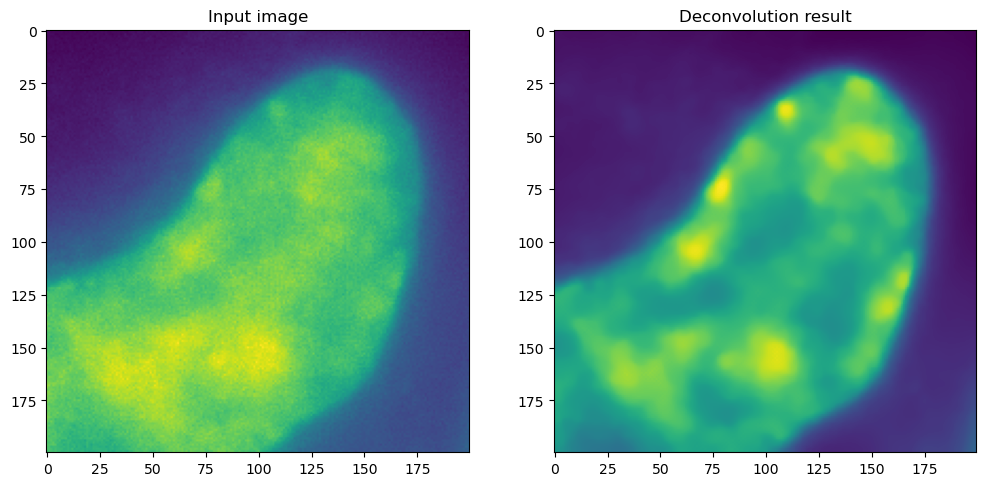
Running the RTLV deconvolution op

With the synthetic PSF we can now deconvolve the input image. The RTLV works on 32-bit images, so before we can use the RLTV op we need to convert the input img to 32-bit.

# convert input image to 32-bit and deconvolve with RTLV
img_f = ij.op().convert().float32(img)
img_decon = ij.op().deconvolve().richardsonLucyTV(img_f, psf, iterations, reg)

# display slice 30 of the input image and deconvolution result side by side
fig, ax = plt.subplots(1, 2, figsize=(12, 9))
ax[0].imshow(ij.py.from_java(img[:, :, 30]))
ax[0].set_title("Input image")
ax[1].imshow(ij.py.from_java(img_decon[:, :, 30]))
ax[1].set_title("Deconvolution result")

# display plot
plt.show()

References

¹: Dey et. al, Micros Res Tech 2006
²: Gibson & Lani, JOSA 1992

References

1: Dey et. al, Micros Res Tech 2006 2: Gibson & Lani, JOSA 1992