Gray Level Co-occurrence Matrices (GLCM)

In this notebook, we will demonstrate how to use Gray Level Co-occurrence Matrices (GLCM), also known as haralick features, to perform texture analysis with PyImageJ. To learn more on GLCM and its applications, please visit the GLCM wikipedia page.

In this example, we will work with a 2D image (shape: (500, 500)) of HeLa cells infected with HIV_NL4-3 expressing mVenus tagged Gag polyprotein. The field of view contains 4 cells, 3 of which are at below the cooperative threshold for Gag assembly (i.e. the concentration of HIV Gag is too low to multimerize into viral particles at the plasma membrane) and 1 cell at or above the assembly threshold¹. This workflow extracts 6 crops from the sample image, 4 crops from each of the cells and 2 crops from the background, and computes the GLCM correlation and difference variance values. By analyzing the texture of the crops from each cell’s cytoplasm we can identify cells in active viral particle production (cell 4) and cells that are expressing the flourescent Gag protein but not yet producing viral particles (cells 1, 2 and 3).

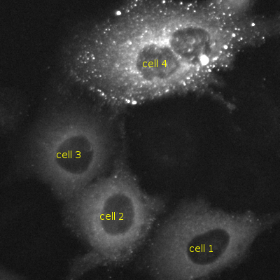
^{Cells 1, 2 and 3 are below Gag assembly threshold and are not making viral particles. Cell 4 is at or above the assembly threshold and is making viral particles.}

Texture analysis with GLCM

The GLCM operation requires 3 parameters, in addition to the input image, that need to be carefully selected.

• Gray levels

• Distance

• Orientation/Angle

Gray Levels

The number of discrete intensity values to bin the image pixel data into. Typically you want to select a value that is smaller than the maximum gray value of the given image as a power of 2. For example, if your image is 8-bit then the maximum gray value (i.e. the maximum value you can store in an 8-bit address) is 255. Therefore, good gray level values for 8-bit images are powers of 2 smaller than 255:

2n	Value
21	2
22	4
23	8
24	16
25	32
26	64
27	128

Distance

The distance a pair of pixels at a given orientation/angle to consider. This value should be adjusted for your dataset. For fine textures start with small pixel distance values (e.g. 2). For coarser details use a larger distance value.

Orientation/Angle

The angle at which pairs of pixels are compared, using the specified pixel distance, to check for co-occurrence. A specific angle can be used for rotationally significant features, or for rotationally invariant features, co-occurrence matrices can be iteratively generated at varying angles and averaged together.

Available GLCM texture analyses in imagej-ops

The imagej-ops framework offers the following GLCM/Haralick feature texture measurements:

• Angular Secondary Moment (ASM)

• Cluster Prominence

• Cluster Shade

• Contrast

• Correlation

• Difference Entropy

• Difference Variance

• Entropy

• Information Measure of Correlation 1 (icm1)

• Information Measure of Correlation 2 (icm2)

• Inverse Difference Moment (ifdm)

• Max Probability

• Sum Average

• Sum Entropy

• Texture Homogeneity

• Variance

Correlation and Difference Variance GLCM textures

This notebook will use two texture measurements: correlation and difference variance. The correlation texture measurement is a measure of linear gray level dependency between a given set of pixels. High correlation values indicate there is a strong linear relationship between the gray levels in the image. Conversely, low correlation values indicate a weak linear relationship. Visually a texture with a higher correlation value indicates a smoother or more uniform texture, while a lower value suggests an image texture with more rapid changes and variations in pixel intensity.

The difference variance texture is a measure of pixel intensity variation between a given set of pixels. High difference variance values indicate that there is significant pixel intensity variation between a given set of pixel gray levels. Low difference variance values indicate that there are fewer transitions between gray level pair values. Visually, a texture with a higher difference variance value may appear noisy, whereas a texture with a lower difference variance value will appear more homogeneous.

With these two textures measurements we can analyze an image and determine how smooth and variable the images are.

Using PyImageJ and imagej-ops for GLCM texture analysis

Let’s start by first initializing ImageJ2 and import the needed Java classes.

import imagej
import matplotlib.pyplot as plt
import pandas as pd
from matplotlib import patches

ij = imagej.init(add_legacy=False)
print(f"ImageJ2 version: {ij.getVersion()}")

ImageJ2 version: 2.14.0

Next we need to import the MatrixOrientation2D Java class which contains angle parameters we can specify. To make it easy to use all four angles (antidiagonal, diagonal, horizontal and vertical), let’s load the MatrixOrientation2D orientations into a list.

# get MatrixOrientation2D Java class
MatrixOrientation2D = imagej.sj.jimport('net.imagej.ops.image.cooccurrenceMatrix.MatrixOrientation2D')

# create orientation list
orientations = [
    MatrixOrientation2D.ANTIDIAGONAL,
    MatrixOrientation2D.DIAGONAL,
    MatrixOrientation2D.HORIZONTAL,
    MatrixOrientation2D.VERTICAL
]

The following cell will set up the run_glcm() and process_crops()functions. The run_glcm() function accepts a single 2D image, obtains the correlation and difference variance GLCM texture values and returns a tuple. The process_crops() function will process a dict of crops we will generate later and feeds each crop to the run_glcm() function. Because this dataset does not have any rotationally significant features, the process_crops() function will iterate through all 4 orientations and average the results before returning a pandas.DataFrame. Once we have the pandas.DataFrame we can easily plot the data on a scattter plot.

def run_glcm(img, gray_levels: int, dist: int, angle):
    """
    Compute the correlation and difference variance GLCM textures from an image.

    :param img: An input ImgPlus
    :param gray_levels: Number of gray levels
    :param dist: Distance in pixels
    :param angle: MatrixOrientation2D angle
    :return: A tuple of floats: (correlation, difference variance)
    """
    # compute correlation and difference variance
    corr = ij.op().haralick().correlation(img, gray_levels, dist, angle)
    diff = ij.op().haralick().differenceVariance(img, gray_levels, dist, angle)
    
    # convert to Python float
    corr = ij.py.from_java(corr)
    diff = ij.py.from_java(diff)

    return (corr.value, diff.value)

def process_crops(crops, gray_levels: int, dist: int) -> pd.DataFrame:
    """
    Process a dict of ImgPlus images with GLCM texture analysis.

    :param crops: A dict of ImgPlus images
    :param gray_levels: Number of gray levels
    :param dist: Distance in pixels
    :return: Pandas DataFrame
    """
    glcm_mean_results = []
    for key, value in crops.items():
        glcm_angle_results = []
        image = ij.py.to_dataset(value) # convert the view to a net.imagej.Dataset
        # compute the correlation and difference variance textures at all orientations
        for angle in orientations:
            glcm_angle_results.append(run_glcm(image, gray_levels, dist, angle))
        # calculate the mean of the angle results
        corr_mean = sum(x[0] for x in glcm_angle_results) / len(glcm_angle_results)
        diff_mean = sum(x[1] for x in glcm_angle_results) / len(glcm_angle_results)
        glcm_mean_results.append((corr_mean, diff_mean))

    return pd.DataFrame(glcm_mean_results, columns=['corr', 'diff'])

We also need to specify the number of gray_levels and the dist before we can perform the texture analysis. Here we selected 128 for gray_levels and a dist of 7 pixels.

# set up GLCM parameters
gray_levels = 128 # a value lower than the bit depth of the image and typically a power of 2
dist = 7 # distance in pixels

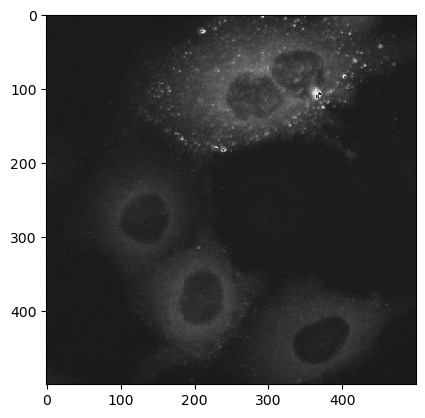
Now let’s load the sample data and view the image.

# load sample data from media.imagej.net
data = ij.io().open('https://media.imagej.net/workshops/data/2d/hela_hiv_gag-yfp.tif')

# convert the net.imagej.Dataset to xarray.DataArray
data_xarr = ij.py.from_java(data)
ij.py.show(data_xarr * 12, cmap='Greys_r') # multiply by 12 to better visualize the data (doesn't change source)

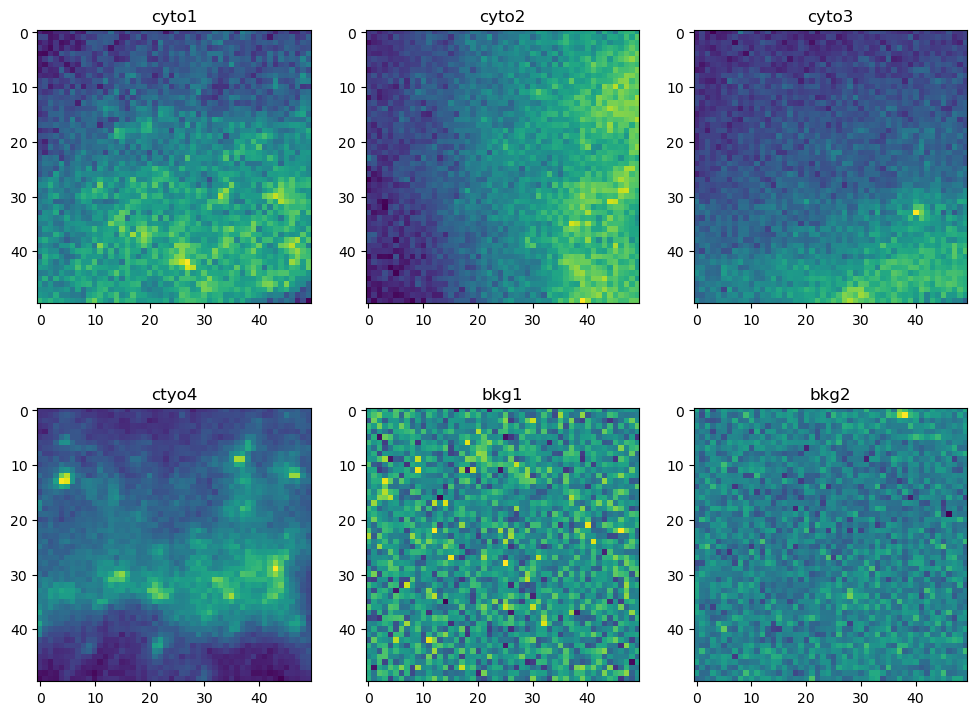
Next we want a total of 6 crops of shape (50, 50) from the input image: 1 crop from each of the four cells, and 2 crops from the background. The exact location of each crop isn’t critical, but a crop should only contain pixels from its particular target. The following cell does 3 things: (1) create a dict of crops by slicing* the original data, (2) create a dict of the min X and min Y coordinates, (3) display the crops in a 2 x 3 matplotlib grid.

*: Slicing a net.imagej.DefaultDataset like we do here to produce crops, returns a view.

# create 50 x 50 crops from the input image (note that these slices are Java objects)
crops = {
    "cyto1": data[318: 368, 369: 419], # cell 1 cytoplasm crop
    "cyto2": data[130: 180, 355: 405], # cell 2 cytoplasm crop
    "cyto3": data[87: 137, 194: 244],  # cell 3 cytoplasm crop
    "cyto4": data[256: 306, 43: 93],   # cell 4 cytoplasm crop
    "bkg1": data[19: 69, 57: 107],     # background 1 crop
    "bkg2": data[263: 313, 221: 271]   # background 2 crop
}

# store the min x and min y values to draw crop boxes
crop_coords = {
    "cyto1": (318, 369),
    "cyto2": (130, 355),
    "cyto3": (87, 194),
    "cyto4": (256, 43),
    "bkg1": (19, 57),
    "bkg2": (263, 221)
}

# view the crops in a 2 x 3 grid in matplotlib
fig, ax = plt.subplots(2, 3, figsize=(12, 9))
ax[0, 0].imshow(ij.py.from_java(crops.get("cyto1")))
ax[0, 0].set_title("cyto1")
ax[0, 1].imshow(ij.py.from_java(crops.get("cyto2")))
ax[0, 1].set_title("cyto2")
ax[0, 2].imshow(ij.py.from_java(crops.get("cyto3")))
ax[0, 2].set_title("cyto3")
ax[1, 0].imshow(ij.py.from_java(crops.get("cyto4")))
ax[1, 0].set_title("ctyo4")
ax[1, 1].imshow(ij.py.from_java(crops.get("bkg1")))
ax[1, 1].set_title("bkg1")
ax[1, 2].imshow(ij.py.from_java(crops.get("bkg2")))
ax[1, 2].set_title("bkg2")

# display the 2 x 3 image grid
plt.show()

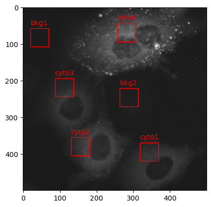
Viewing the crops in a 2 x 3 grid is helpful, but its hard to determine where these particular crops are extracted from in the original image. The next cell will display the original input image with red boxes indicating the location each crop was extracted from.

# display the original image (multiplied by 12 to increase it's brightness)
plt.imshow(data_xarr * 12, cmap='Greys_r')

# create red boxes for each crop on top of the original image
for key, value in crop_coords.items():
    x = value[0]
    y = value[1]
    rect = patches.Rectangle((x, y), 50, 50, linewidth=1, edgecolor='r', facecolor='none')
    plt.gca().add_patch(rect)
    # add a label above each box
    plt.text(x + 25, y - 15, key, color='r', ha='center', va='center')

# display the original image with red crop boxes
plt.show()

Finally, we can now perform the correlation and difference variance GLCM texture analysis. This last cell uses the process_crops() function that we setup earlier, which processes each crop in the crops dictionary with the run_glcm() function. The output pandas.DataFrame is then plotted on a matplotlib scatter plot.

# set plot style
plt.style.use('ggplot')

# process the dict of crops and add crop names to the output dataframe
df = process_crops(crops, gray_levels, dist)
df["name"] = ["cyto1", "cyto2", "cyto3", "cyto4", "bkg1", "bkg2"]

# plot the data in a matplotlib scatter plot
plt.scatter(df['corr'], df['diff'])

# add labels
for i in range(len(df)):
    plt.annotate(f"{df['name'][i]}", (df['corr'][i], df['diff'][i]))

# add labels and title
plt.xlabel('corr')
plt.ylabel('diff')
plt.title('GLCM texutre plot')

# display the scatter plot
plt.show()

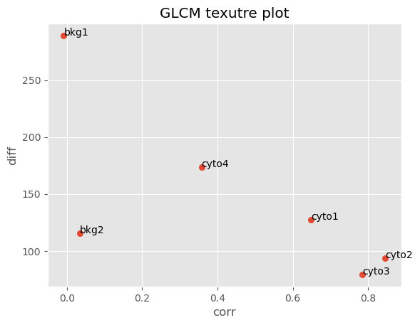
In the resulting scatter plot we can clearly see that our crops clustered in descrete regions. Crops cyto1, cyto2 and cyto3 which all come from the cytoplasm of cells expressing mVenus-Gag below the Gag multimerization threshold (i.e. these cells are not making viral particles) clustered in a region with high correlation and low difference variance values, indicating that these images are smooth and invariant. Crops bkg1 and bkg2 are extracted from the background. Interestingly, while they appear visually smooth they have a low GLCM correlation value indicating they are infact not homogenous. The difference variance values for bkg1 and bkg2 suggests bkg1 is more variable in signal inensity than bkg2. Looking back at the 2 x 3 grid of crops we made earlier, we can see that indeed bkg1 and bkg2 are not homogenous and bkg1 appears more noisy than bkg2. Lastly crop cyto4, which was extracted from the cell at or above the Gag multimerization threshold (i.e. the cell is producing viral particles) has a lower correlation value than cyto1, cyto2 and cyto3 but a higher value than bkg1 and bkg2. This suggests that cyto4 is not as smooth as the other cells but smoother than the background.

By measuring the GLCM correlation and difference variance textures we can distinguish cells that are in the assembly stage of the viral life cycle and are producing viral particles and those that are not.

References

¹: Becker et. al, J Virol 2017